- Other Fluke companies:
- Fluke
- Fluke Biomedical
- Fluke Networks
- Fluke Process Instruments
See more Fluke brands

Calibration by characterization
Tolerance testing
There are two types of calibrations applicable to PRTs—characterization and tolerance testing. The type of calibration to perform is determined by the way in which the Unit Under Test (UUT) is to be used and the accuracy required by the user. Characterization is the type of calibration in which the UUT resistance is determined at several temperature points and the data are fitted to a mathematical expression. Tolerance testing on the other hand is a calibration in which the UUT resistance is compared to defined values at specific temperatures. No data fitting is performed. In the laboratory, we are required to perform both types of calibration depending upon our customer’s needs.
Characterization is the method that is most often used for medium to high accuracy PRT calibration. With this method, a new resistance vs. temperature relationship is determined anew with each calibration. Generally, with this type of calibration, new calibration coefficients and a calibration table are provided as a product of the calibration. There are five basic steps to perform as listed below:
All temperature sources have instabilities and gradients.These translate into calibration errors and/or uncertainties. To minimize the effects, the probes should be placed as close together as practical. In baths the probes to be calibrated should be placed in a radial pattern with the reference probe in thecenter (focus) of the circle. This ensures an equal distancefrom the reference probe to each of the UUTs.In dry-well temperature sources, the reference probeand probes to be calibrated should all be placed thesame distance from the center for best results, butthe reference may be placed in the center if needed.
Also, the sensing elements should be on the same horizontal plane. Even though sensing elements are different lengths, having the bottoms of the probes at the same level is sufficient. Sufficient immersion must be achieved so that stem losses do not occur. Generally, sufficient immersion is achieved when the probes are immersed to a depth equal to 20 times the probe diameter plus the length of the sensing element. For example, consider a 3/16 inch diameter probe with a 1 inch long sensing element. Using the rule of thumb, 20 x 3/16 in + 1 in = 3 3/4 in + 1 in = 4 3/4 in. In this example, minimum immersion is achieved at 4 3/4 inches. This rule of thumb is generally correct with thin wall probe construction and in situations of good heat transfer. If the probe has thick wall construction and/or poor heat transfer is present (such as in the case of a dry-well with incorrectly sized holes), more immersion is required.
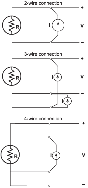
This step is straightforward. Connections must be tight and in proper 2-, 3-, or 4-wire configuration. If using 4-wire configuration, ensure that the current and voltage connections are correct. See Figure 1.
There are two ways to measure the reference probe and determine the temperature. Both techniques have the same potential accuracy. That is, if done correctly, neither technique is inherently more accurate than the other.
The first and best method is used with sophisticated readouts designed for temperature work. The resistance is measured and the temperature calculated from calibration coefficients which were entered into the readout previously. Once these calibration coefficients have been entered, the temperature calculations are accomplished internally and the readout displays in temperature units. The temperature data is available in real time. Some modern readouts also display the data in graphical format, allowing the operator to determine stability at a glance. Both of these features speed up the process and eliminate possible operator error due to incorrect table interpolation.
The second method is used when the readout does not provide for proper temperature calculation. (Some readouts, particularly DMMs, have some of the more popular temperature conversions built in. These typically do not allow use of unique calibration coefficients and cannot be used for accurate temperature calibration.) In this case, the resistance is measured and the temperature is determined from either a calibration table or from a computer or calculator program.
Since the temperature must be calculated after the resistance is measured, the process is slower and does not provide immediate, real time temperature data. See Tables 1 and 2 below.
Table 1. Interpolation from an RTD calibration table (resistance vs. temperature).
| t( °C) | R(t) (Ω) | dR/dt(t) Ω/°C |
| 400 | 249.8820 | 0.3514 |
| 401 | 250.2335 | 0.3513 |
| 402 | 250.5848 | 0.3512 |
| 403 | 250.9360 | 0.3511 |
| 450 | 267.3108 | 0.3456 |
| 451 | 267.6564 | 0.3455 |
| 452 | 268.0019 | 0.3452 |
| 453 | 268.3472 | 0.3452 |
| 1. Measure the reference probe resistance | 249.9071 Ω |
| 2. Locate where it falls on the table | between 249.8820 Ω and 250.2335 Ω |
| 3. Subtract lower table value from measured value | 249.9071 Ω – 249.8820 Ω = 0.0251 Ω |
| 4. Divide by dR/dT(t) (slope of curve) | 0.0251 / 0.3514 = 0.0714 °C |
| 5. Add fractional temperature to table value | 0.0714 ’C + 400 = 400.0714 °C |
Table 2. Interpolation from an RTD calibration (resistance ratio (W) table).
| t( °C) | W(t) | dt/dW(t) |
| 300 | 2.1429223 | 275.2199 |
| 301 | 2.1465557 | 275.3075 |
| 302 | 2.1501880 | 275.3951 |
| 303 | 2.1538192 | 275.4827 |
| 350 | 2.3231801 | 279.6655 |
| 351 | 2.3267558 | 279.7559 |
| 352 | 2.3303304 | 279.8464 |
| 353 | 2.3339037 | 279.9369 |
| 1. Measure reference probe resistance | 54.75258 Ω |
| 2. Calculate W (Rt/Rtpw) (Rtpw = 25.54964) | 54.75258 Ω / 25.54964 Ω = 2.1429883 |
| 3. Locate where it falls on the table | between 2.1429223 and 2.1465557 |
| 4. Subtract lower table value from measured value | 2.1429883 – 2.1429223 = 0.000066 |
| 5. Multiply by dt/dW(t) (inverse slope of curve) | 0.000066 • 275.2199 = 0.0182 °C |
| 6. 6) Add fractional temperature to table value | 0.01821 °C + 300 °C = 300.0182 °C |
Since the UUTs are resistance thermometers similar to the reference probe, they are measured in a similar manner. If several UUTs are undergoing calibration, ensure that when they are connected or switched in, sufficient time is allowed for self-heating to occur before the data is recorded. Also, ensure that the readout is set to the correct range to provide the proper source current and to prevent range changes between the measurements at different temperatures. Typically, the measurements are conducted starting at the highest temperature of calibration and working down. Additionally, it increases the precision of the calibration to use a mean (average) value calculated from multiple measurements at the same temperature. Often, the readout is designed with statistical features to facilitate this practice. It is also a good practice to close the process with an additional measurement of the reference probe. The sequence in which the probes (reference and UUT) are measured is referred to as a measurement scheme. There are many variables to consider when designing a measurement scheme. Some points to consider are:
It is not possible for us to anticipate all of the variables and discuss the optimum solutions here. However, in the following examples, we will consider some typical calibration scenarios and suggested measurement schemes.
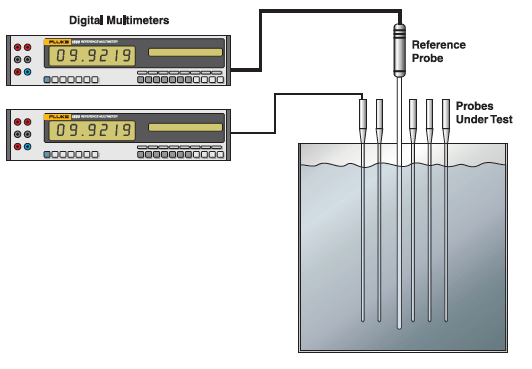
The reference probe is connected to one readout and the first UUT is connected to the second readout. This places the probes to be measured under current at all times, thus, eliminating self-heating errors caused by changing current conditions. The UUTs will be connected and measured individually.
The scheme is as follows:
REF(1)-UUT (1) - REF(2)-UUT (2) - REF(3)-UUT (3) - REF(4)-UUT (4) - REF(5)-UUT (5)
This provides 5 readings each of the reference and the UUT. Take the average of the readings and use it for the data fit. If the reference probe readings are in resistance, the temperature will have to be computed. After completion, repeat the process for the additional UUTs.
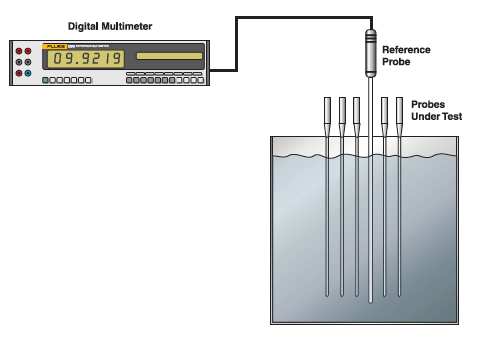
This example is similar to the first except that the reference probe and UUT must be measured by the same readout. The same scheme can be followed but more time must be allowed between readings to allow for self-heating. Since more time is involved, it might be beneficial to reduce the number of readings from five to three unless the heat source is extremely stable. Each probe will be connected and measured individually
The scheme is as follows:
wait-REF(1)-wait-UUT (1) - wait-REF(2)-wait-UUT(2) - wait-REF(1)-wait-UUT(3)-done
This provides 3 readings each of the reference and the UUT. Take the average of the readings and use it for the data fit. Again, the reference probe readings are in resistance so the temperature will have to be computed. After completion, repeat the process for the additional UUTs.
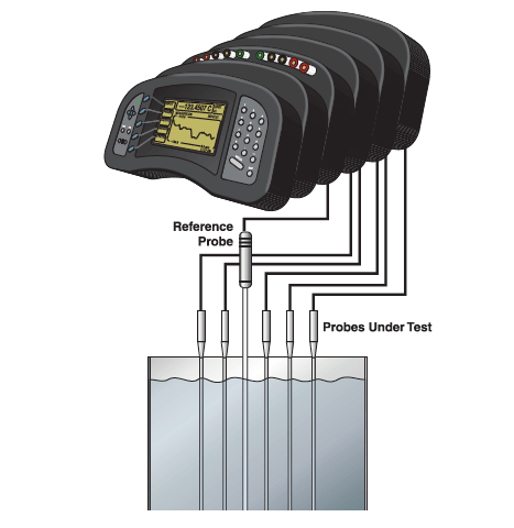
In this example, all of the probes are connected directly to the thermometer readout, a Fluke Calibration 1560 Black Stack. The readout controls the measurement and scans through all probes performing statistics in real time. Current may or may not be supplied at all times depending on the type of thermometer readout. If current is supplied at all times, there will be no self-heating errors. If current is not supplied at all times, ensure that the switching is done rapidly enough to reduce self-heating errors to a negligible level.
The scheme is as follows
REF - UUT 1 - UUT 2 - UUT 3 - UUT 4 - UUT 5 - repeat 10 or more times
This provides many readings each of the reference and all of the UUTs. The average can be calculated and displayed directly by the readout. Also, the reference probe readings are in temperature so no further computation is required - the data is ready to fit.
Data fitting is simple in concept but can be complicated in practice. Essentially it is a process of solving a set of simultaneous equations which contain the calibration data to arrive at a set of coefficients unique to the PRT and calibration. There are several commercial software programs available specifically written to accomplish this task. Some are limited in function and do no more than solve the basic temperature functions. Others are more flexible and allow options regarding the number and location of calibration points and provide analysis regarding the precision of the resultant fit. The latter type of program is preferred. For metrologists who wish to tackle the algorithms themselves, a good mathematics application software like Mathcad or Mathematica or even a spreadsheet like Excel is extremely helpful. Fluke Calibration offers two programs: TableWare for calculating calibration coefficients and MET/TEMP II for automating calibration tasks and calculating calibration coefficients. Of course, programs can be written in any of the modern computer languages (with double precision or better floating point capability) to perform the calculations with equal accuracy.
There are several equations which are used for PRT characterization. Among the most common are the International Temperature Scale of 1990 (ITS-90) series, the Callendar-Van Dusen, and third through fifth order polynomials. Obviously, with more than one model available to describe the behavior of a physical system, we must choose which one is best for our situation. The following discussion covers the features and purpose of each of these models and describes the form of the equations. The steps necessary to actually fit the data will be discussed in the section on mathematics later in this manual.
ITS-90: The ITS-90 series of functions were developed through a concerted effort from the international metrology community’s leading temperature experts. These functions are intended to describe how the behavior of the SPRT relates, with a very high degree of precision, to the fixed points on which the scale is based. It does this extremely well SPRTs and with high quality PRTs. The ITS-90 uses a reference function— deviation function structure that has many advantages over traditional polynomials and is the preferred model for high accuracy applications. In the equations below, capital T refers to ITS-90 temperatures expressed in Kelvin units.
Where:
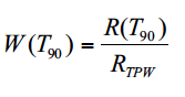
W(T90) = resistance ratio at temperature T
R(T90) = measured resistance at temperature T
RTPW = measured resistance at the triple point of water
Where:
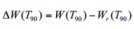
ΔW(T90) = deviation of calculated W from reference function at temperature T
W(T90) = calculated resistance ratio at temperature T (from equation (1))
Wr(T90) = reference function value at temperature T
Where:
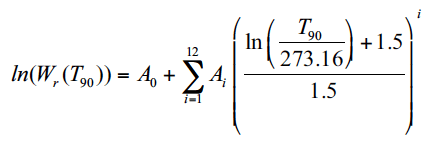
Wr(T90) = reference function value at temperature T
Ai = reference function coefficients from definition
Where:
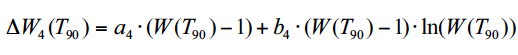
ΔW(T90) = calculated deviation value at temperature T (from equation (2))
W(T90) = calculated resistance ratio at temperature T (from equation (1))
a4, b4 = resulting calibration coefficients
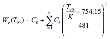
Where:
Wr(T90) = reference function value at temperature T
Ci = reference function coefficients from definition
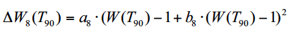
Where:
ΔW(T90) = calculated deviation value at temperature T (from equation (2))
W(T90) = calculated resistance ratio at temperature T (from equation (1))
a8, b8 = resulting calibration coefficients
The designations 4 and 8 in the deviation functions, equations (4) and (6) were inserted by NIST for identification of specific subranges. The values for the coefficients Ai and Ci in the reference functions, equations (3) and (5) are given in Table 3.
Table 3. ITS-90 Reference Function Coefficients
| Coefficient | Value |
| A0 | -2.135 347 29 |
| A1 | 3.183 247 20 |
| A2 | -1.801 435 97 |
| A3 | 0.717 272 04 |
| A4 | 0.503 440 27 |
| A5 | -0.618 993 95 |
| A6 | -0.053 323 22 |
| A7 | 0.280 213 62 |
| A8 | 0.107 152 24 |
| A9 | -0.293 028 65 |
| A10 | 0.044 598 72 |
| A11 | 0.118 686 32 |
| A12 | -0.052 481 34 |
| C0 | 2.781 572 54 |
| C1 | 1.646 509 16 |
| C2 | -0.137 143 90 |
| C3 | -0.006 497 67 |
| C4 | -0.002 344 44 |
| C5 | 0.005 118 68 |
| C6 | 0.001 897 82 |
| C7 | -0.002 044 72 |
| C8 | -0.000 461 22 |
| C9 | 0.000 457 24 |
Callendar-Van Dusen: The Callendar-Van Dusen (CVD) equation has a long history. It was the main equation for SPRT and PRT interpolation for many years. It formed the basis for the temperature scales of 1927, 1948, and 1968. This equation is far simpler than the ITS-90 equations but has serious limitations in the precision of fit. As a result, it is not suitable for high accuracy applications but is perfectly suited to modest accuracy applications. Partly due to its history and simplicity, but mostly due to its continued suitability, it continues to be the preferred model for industrial platinum resistance thermometers today. In the equations below, lower case t refers to ITS-90 temperature in Celsius units.
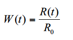
Where:
W(t) = resistance ratio at temperature t
R(t) = measured resistance at temperature t
R0 = measured resistance 0 °C
And...
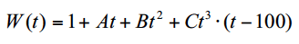
Where:
W(t) = resistance ratio at temperature t (reference 0 °C)
A,B,C = calibration coefficients (C is = 0 for temperatures above 0 °C)
Note:
All temperatures are expressed in °C and the resistance ratio (W) is referenced to 0 °C rather than the triple point of water (0.010 °C) as with the ITS-90.
Polynomials: Polynomials are frequently used to model physical phenomena from all fields of science. They have limited use with PRTs because of the high order required to achieve a suitable fit. (Recall that the reference functions for the ITS-90 are 9th and 12th order polynomials for the ranges above 0 °C and below 0 °C.) Additionally, the previous models use resistance ratio as the variable to fit. Most polynomials in use fit the resistance directly. Since resistance is not as stable as the resistance ratio, these models have serious limitations. That having been said, polynomials can be very useful over limited ranges and in applications where accuracy requirements are very modest.
Where:
t = temperature
R = resistance
a,b,c,d,e = calibration coefficients
Tolerance testing method
PRT calibrations involving tolerance testing are reserved for low accuracy applications. With this type of calibration the UUT resistance is compared to defined values at specific temperatures. The values are defined by one of the common models such as the ASTM 1137 or IEC 60751 curve. PRTs calibrated in this way are generally used in industrial style applications where the readout is unable to accept unique coefficients but is pre-programmed with a common PRT curve. The probe must be tested to ascertain its compliance to the curve of interest. There are accuracy classes defined that probes are intended to fit.
The two common accuracy classes are class A and class B:
| IEC 60751 | ASTM 1137 | |
| Class A | ± [0.15 + (0.002 · t)] °C | ± [0.13 + (0.0017 · t)] °C |
| Class B | ± [0.30 + (0.005 · t)] °C | ± [0.25 + (0.0042 · t)] °C |
These include errors arising from deviations in R0 and from errors in slope. Frequently, we will see probes rated at a fraction of Class A. For example, 0.1 ASTM Class A. Fractional accuracy is achievable in sensors alone, but are very difficult to achieve in probes. The calculations are straightforward. See below:
Example 4: Calculate the accuracy of a 0.1 ASTM Class A probe at 100 °C
1. = (0.13 + (0.0017 · t)) · 0.1
2. = (0.13 + (0.0017 · 100)) · 0.1
3. = (0.13 + 0.17) · 0.1 = 0.03
PRTs that conform to a standard specification such as ASTM 1137 or IEC 60751 are expected to be within tolerances of defined resistance values for any given temperature. The resistance values are defined by a form of the Callendar-Van Dusen (CVD) equation and specified values for coefficients A,B and C (see table 4). These values may be determined using a published table or calculated by solving the equations.
Measurements for tolerance testing are carried out in the same manner as measurements for characterization. ITS-90 temperature is determined by the reference thermometer. The resistance of the UUT is then compared to the defined resistance values, and pass or fail status is determined based on the specified tolerances (i.e. Class A or Class B).
Table 4. Equations for ASTM 1137 and IEC 60751
| Range | Callendar-Van Dusen Equation |
| −200 ° C t ⟨ 0 °C | Rt = R0[1 + At + Bt2 + C(t - 100)t3] |
| 0 ° C ≤ t ≥ 650 °C | Rt = R0[1 + At + bt2] |
| ASTM 1137 and IEC 60751 coefficient values | |
|
A = 3.9083 X 10⁻³ B = –5.775 X 10⁻⁷ C = –4.183 X 10⁻¹² |
|
Example 5: Calculate the tolerance of a 0.1 ASTM Class A probe at 100 °C
| Measure the reference probe temperature | 100.00 °C |
| Measure the indicated UUT temperature using ASTM 1137 equation and coefficients | 100.05 °C (Given) |
| Calculate the error | 0.05 °C |
| Calculate the tolerance at 100.00 °C | 0.03 °C (See example 4) |
| Determine tolerance status | Fail (0.05 °C > 0.03 °C) |
To be certain of the tolerance status of a calibrated instrument it is necessary to have calibration uncertainties that are significantly better than the tolerance of the instrument being calibrated. Typically a ratio of 4:1 or four times better than the tolerance of the instrument being calibrated is required. When this is not the case the risk may be unacceptably high that out of tolerance instruments will be falsely accepted or that in tolerance instruments will be falsely rejected. As the magnitude of the detected error approaches the tolerance of the calibrated instrument, the risk of incorrectly assigning a tolerance status increases. Guard bands may be helpful in these circumstances. For example if a guard band is 80 % of the tolerance then instruments found within 80 % of their tolerance will pass, instruments outside of the tolerance will fail and instruments that are in between will be indeterminate. The better the calibration uncertainties the tighter the guard band can be.
Platinum Resistance Thermometer calibration procedures are similar whether the method selected is characterization or tolerance testing. For best accuracy with modern equipment choose characterization. For equipment that does not allow characterization, tolerance testing may be your only choice and this is a common situation in industry today. When conducting tolerance testing it is important to use equipment and procedures with sufficient accuracy to determine the tolerance status confidently.
Platinum Resistance Thermometers (PRTs)
Platinum Resistance Thermometers (PRT) (App Note)
Selecting a dry-block calibrator (Blog)
How to do a temperature sensor comparison calibration (Blog)
Annealing a PRT: Why, When and How (Webinar)
How to calibrate your PT100 temperature sensor and other probes in-house (Blog)
Speak with a calibration product expert about your probe and equipment needs